All published articles of this journal are available on ScienceDirect.

The Effect of Financial Development on CO2 Emissions: A Nonlinear Dynamic Panel Data Analysis
Abstract
Aim
This study aimed to find out if it is possible to utilize the financial system and/or instruments to improve environmental quality.
Background
Since the Industrial Revolution, there has been rapid global warming and climate change due to the use of fossil fuels, which produce greenhouse gas emissions due to economic activities that do not involve environmental sensitivity.
Method
To analyze the effect of financial development on CO2 emissions, we developed a nonlinear hypothesis by combining four hypotheses of carbon-friendly financing, carbon financing, pollution haven, and pollution halo. To test the validity of the hypothesis, we employed nonlinear system GMM analysis.
Result
We found an inverse U-curve relationship between financial development and CO2 emissions, supporting the nonlinear hypothesis for 120 countries over the period of 1999-2019.
Conclusion
Below the specific threshold, financial development has a significantly positive effect on CO2 emissions if carbon-friendly financing is followed in underdeveloped financial systems, and above the specific threshold, financial development has a significantly negative effect on CO2 emissions in well-developed financial systems. Beyond empirical analysis, the theory also introduces the concept of a 'financial trap', suggesting that the minimum achievable level of CO2 emissions in countries with underdeveloped financial systems is consistently higher than that of countries with well-developed financial systems.
1. INTRODUCTION
In pursuit of the ideal economic development, humanity has been destructive to the environment due to its reckless consumption of resources over the centuries of its rapid progress (Feltz, 2019). Since the Industrial Revolution, there has been rapid global warming and climate change due to the use of fossil fuels, which produce greenhouse gas emissions due to economic activities that do not involve environmental sensitivity. Many scientists argue that the effects of climate change can be devastating, and poses an existential threat to human civilization. This global ecological crisis, linked to the motivation for continuous growth, has led to a new vision of development centered on environmental protection (Riedy, 2016).
In today’s industrialized world, transportation, factory chimneys, fossil fuel production, motorized vehicles using fossil fuels, agricultural activities, etc., all contribute to environmental pollution due to higher CO2 emissions.
This new perspective on development emerged as social scientists increasingly turned their attention to the challenges posed by climate change. It is based on the idea of resource sustainability and looks at what steps can help people move ahead economically while also being good for the environment (Riedy, 2016).
The impact of economic development on environmental quality is multidimensional, complex, and country-specific (Riedy, 2016). For example, many variables that are determinants of economic development, such as ‘fixed capital investment’, ‘energy consumption’, ‘urbanization’, and ‘financial development’ are also variables that affect the environmental quality (Munasinghe, 2003; Jiang & Ma, 2019; Abid et al., 2022).
Greenhouse gas (GHG) emissions were supposed to decline by 20% in the European Union. This target was part of a plan called the European 20/20/20 Objectives, having three goals, i.e., using 20% more renewable energy by 2020, becoming 20% more energy efficient, and lowering CO emissions by 20%.
As a result of financial globalization, there have been fewer physical barriers between financial markets and economic activity. This trend has made the financial system more important because it collects people's savings and uses extra money to make investments and meet businesses' cash flow needs (Syed Anees Haider Zaidi, 2019). In this process, the use of various financial instruments has increased, and the structure of the financial system has expanded. This issue, called financial development, has come to the fore as a significant determinant of economic development (Levine, 2004; Kegley & Blanton, 2014; Levine, 2012).
Financial development often runs parallel to the development and modernization of industry in a country and can also be a source of environmental problems. Particularly in societies in the early stages of development, banks, insurance companies, and other financial institutions are eager to lend, borrow, and invest in energy, mining, and other sectors because of their perception of risk and expectations of profitability. Due to this, activities, like coal mining, and processes employed in the oil industry can lead to environmental problems, like carbon dioxide emissions and water pollution (Zhang, 2011; World Bank, 2021).
On the other hand, issues, such as increased energy use, proliferation of industrial activities, and increased need for transportation reinforce environmental problems. In addition, the increase in carbon emissions is one of the most important causes of climate change (Sadorsky, 2010).
Many countries support efforts made by the financial system to encourage investments in order to enhance financial development. At a certain stage of the development process, environmental awareness, pressure from advocate groups, and national and international commitments and regulations are the factors that increase environmental sensitivity. In addition, issues, such as climate crisis and air pollution, which reduce people's quality of life and cause financial losses, as well as resource sustainability, are also factors that favor environmentally friendly policies (Raza & Shah, 2018).
In other words, it is possible to utilize the financial system and/or its instruments to improve environmental quality. Banks can help improve the environment and solve environmental problems by supporting investments that are good for the environment, stopping people from using money to fix environmental problems, and giving investors the chance to use their money to support projects that are good for the environment (Abbasi & Riaz, 2016).
Financial regulations may encourage financial institutions to finance environmentally friendly investments or impose restrictions on the financing of activities that cause environmental problems. Green financing practices, which means that financial institutions invest in environmentally friendly projects, are also an important instrument that can be used to reduce the environmental problems caused by financial development. Green financing, which can encourage investments in areas, such as the transition to renewable energy sources, energy efficiency, and waste management, can reduce environmental problems and support sustainable development (Sachs et al., 2019).
Additionally, we can use various tax incentives to support environmentally friendly investments. In addition, financial institutions can offer environmentally friendly financial products, such as green bonds and funds, to encourage investors to engage in ecologically sustainable investments (Elkins & Baker, 2001; OECD, 2015).
As can be seen, the impact of financial development on carbon emissions and, more broadly, on environmental quality is complex. Financial development can directly and indirectly cause carbon emissions, but it can also be used to support environmental sustainability. The relationship between the variables varies depending on the policies and investment areas.
In his meta-regression analysis, Gök (2020) found a significantly positive effect of financial development on CO2 emissions and concluded that the effect of financial development on carbon emissions varies in both magnitude and direction depending on which financial development indicator is used, which estimation technique is used, which country or region is included, and which period is analyzed (Liu et al., 2023; Manta et al., 2020; Sehrawat & Giri, 2014).
Therefore, it is possible to find positive or negative effects. However, we argue that the altering effect is caused by the nonlinear relationship between financial development and CO2 emissions. The current paper investigated why this effect alters and analyzed whether it changes concerning the level of financial development above and below a specific threshold. This investigation can mainly contribute to the relevant literature.
The structure of the following paper is as follows: the next section presents a theoretical perspective, the third section introduces the empirical analysis, and the last section provides the conclusion.
2. THEORETICAL PERSPECTIVE
An extensive literature examines the relationship between financial development and environmental quality/carbon emissions. Some studies (Khan, Hossain, & Chen, 2021; Omri et al., 2015) have found no link between the variables. Other studies have found that financial development may have different effects on environmental quality (Maji, Habibulah, & Saari, 2017; Fu et al., 2022; Sunday Adebayo et al., 2023).
The findings frequently obtained in the literature point to two types of relationships between variables. Financial institutions in countries at early stages of financial development contribute to declining environmental quality because their service policies do not consider carbon emissions. In other words, in the early stages of financial development, the financial system that encourages carbon-emitting industries to continue their current activities increases carbon emissions and negatively affects the environmental quality (Boutabba, 2014).
The studies propose a variety of explanations for these issues. The most basic idea refers to an increase in carbon emissions due to the increase in energy demand with financial development and the increase in dependence on fossil fuels to meet this demand. Another issue is the increase in carbon emissions directly related to the intensification of industrial activities and the expansion of trade due to financial development (Acheampong, 2019; Kirikkaleli, Güngör & Adebayo, 2022).
Another mechanism is that financial development increases industrial production by providing more investment and credit opportunities for activities with high carbon footprints (energy, transportation, logistics infrastructure investments, etc.) through instruments that provide financing for activities that cause negative environmental impacts and even by encouraging foreign direct investment (FDI) in this field. Again, changes in finance lead to more FDI, which boosts economic growth, and more carbon emissions as cities grow (Tamazian & Rao, 2010; Yang et al., 2023; Kahouli, 2017; Xu et al., 2022).
Another reason is that households and firms, which have access to cheap credit due to financial development, turn to expensive goods and services (white goods, refrigerators, automobiles, air conditioners, etc.) that require more use of fossil fuel. In addition, increased transportation demand thanks to the potential income generated by credit expansion also increases energy consumption and thus carbon emissions (Yang et al., 2023; Acheampong, 2019; Abbasi & Riaz, 2016).
It is also suggested that economic actors who accumulate wealth through an advanced financial system, one that enables effective risk diversification, are more likely to pursue new, collective investments at lower individual costs within this climate of confidence. This can boost economic growth at the cost of more carbon emissions and energy use (Sadorsky, 2010; Fung, 2009).
Another reason that encourages environmental degradation due to financial development is that the financial system does not and/or cannot provide sufficient resources for green investments and ignores environmental problems, thus negatively affecting environmental quality (Schmidheiny & Zorraquin, 1996).
Thus, it needs to be considered as to what are the reasons for a country to have the financial structure to support carbon emissions, or even to explicitly encourage them. There may be many political, economic, social, or environmental reasons for this situation. However, the literature generally explains these issues through the lens of the “pollution haven” hypothesis (Mert & Caglar, 2020; Duan & Jiang, 2021). This hypothesis states that with the increase in globalization and international trade, foreign direct investments/companies flee from countries with stricter environmental regulations and prefer countries with less stringent environmental regulations to carry out their industrial activities. This situation, which reduces the production costs of companies, increases the production capacity and employment opportunities of the country, but causes environmental impacts to be transferred to another country and environmental problems to globalize (Thanh, Chin & Nguyen, 2022; Udeagha & Breitenbach, 2023).
Some important studies that have come to this conclusion are the ones carried out by Liu et al. (2022), Shahbaz, Abosedra, & Sbia (2013), Moghadam & Dehbashi (2018), and Zhang (2011). These studies, along with the ones we have already talked about, have led us to our first hypothesis, which is as follows:
Hypothesis 1: Financial development, through carbon-friendly financing, significantly reduces CO emissions below the threshold in underdeveloped financial systems.
However, depending on the sectors to invest in, the amount of investment, and the investment strategy, the environmental impacts of financial development may vary. Studies that have looked at this relationship have also tested the idea that financial growth can help fight climate change and lower carbon emissions by investing in green technologies, using more renewable energy, and providing a lot of resources at different prices during the shift to a low-carbon economy (Shahbaz, 2013; Li, Xu & Zhao, 2023).
Financial development can lead to improved environmental quality in several ways. The first is that financial development provides more resources for the development and use of environment-friendly renewable and efficient R&D technologies and reduces carbon emissions by reducing fossil fuel consumption (Acheampong, Amponsah & Boateng, 2020).
Another reason is that financial development can provide more resources for the use of sustainable production methods, thereby reducing carbon emissions by leading to less energy consumption and less waste production. In addition, carbon taxes can provide more resources for the development and implementation of better public policies, such as emissions trading or renewable energy incentives, which in turn can reduce carbon emissions (Zaidi et al. 2019).
Listed companies, which are under the strict supervision of financial authorities and the public, strive to create a positive image by using environmentally friendly technologies, a factor that can help reduce carbon emissions (Jiang and Ma, 2019). Improved institutional governance also contributes to improved environmental quality through improved regulations (Ofori et al., 2023).
Another factor that promotes environmental quality in the country and enables the financial structure to support such projects is the “pollution halo” hypothesis. This hypothesis claims that investing in developed country companies contributes to the reduction of emissions in the host country because their production structure is based on green technology, unlike the current production of the host country. In other words, FDI in a country leads to the transfer of environment-friendly technology and management methods, which in turn reduces carbon emissions and environmental pollution in the country (Mert & Caglar, 2020; Benzerrouk, Abid & Sekrafi, 2021).
Moreover, with the development and deepening of the financial system, new financial instruments, such as sustainable finance and green finance, have emerged recently. These structures are investment instruments that encourage the transition to sustainability and environment-friendly practices and aim to finance environment-friendly investment projects.
‘Green financing’ refers to these types of financial tools that are used by different groups, like governments and financial institutions, to pay for projects, like lowering carbon emissions, protecting natural resources, managing water, making environmental rules more consistent, and investing in renewable energy sources. They are also meant to give investors the chance to invest their money into projects that have less of an impact on the environment, essentially helping to improve the quality of the environment (Lindenberg, 2014).
Debt instruments under green financing, such as green bonds used to finance environmentally friendly projects, can be issued in advance by public or private actors to raise capital or refinance for ecologically beneficial projects, which is one of the positive effects of financialization on carbon emissions (Kaminker, 2015). Similar to other green financial instruments, green credit supports environmental quality by financing borrowers' income only for projects that make a significant contribution to an environmental goal (WB, 2021).
Like ‘green financing’, another type of financing used to combat climate change is ‘carbon financing’. Carbon credits, also known as carbon allowances, work like permits for carbon emissions. When a company buys a carbon credit from the government, it receives permission to produce one ton of carbon emissions. Once this credit is used, it becomes an offset and cannot be traded again. However, organizations that eliminate or reduce their greenhouse gas emissions can sell carbon emission permits (carbon credits), and companies that need to emit carbon can buy these rights to offset their greenhouse gas emissions, thus leading to improved environmental quality (UNDP, 2022).
Based on the mechanisms mentioned above and the findings of Khan, Khan & Muhammad (2021), Emenekwe, Onyeneke & Nwajiuba (2022), Shahbaz et al. (2013), Stern (2007), Beck & Levine (2005), and Grossman & Krueger (1995), which are among the important studies with results in this direction, helped formulate our second hypothesis as follows:
Hypothesis 2: Above the threshold, financial development has a significant negative impact on CO emissions, similar to carbon financing, in well-developed financial systems.
Countries with underdeveloped financial systems cannot achieve the lowest level of CO2 emissions, even if they improve their financial systems until they reach the threshold level, which is defined as a financial trap. Therefore, the lowest CO2 emission level in countries with underdeveloped financial systems is always higher than the CO2 emission level in countries with well-developed financial systems (Fig. 1).
3. EMPIRICAL ANALYSIS
3.1. Data and Variables
Appendix 1 includes the list of 120 countries that were analyzed in this study. The rationale was to include as many countries as possible to show the nonlinear effect of differing levels of financial development.
Appendix 2 provides the source of the data, while Appendix 3 provides descriptive statistics. Since the data on governance began in 1996 and the data on CO2 emissions concluded in 2019, the analysis spanned the years 1996 to 2019. Hence, the descriptive statistics, cross-section dependency test, and unit root analyses covered the period of 1996-2019 for 120 countries for which the data were available (Appendix 4).
According to the cross-section dependency test provided in Appendix 5, the variables of control of coc and democ were insignificant, meaning that they did not involve cross-section dependence. Hence, we employed the first-generation unit root test for them. And for the rest of the significant variables, we employed a second-generation unit root test.
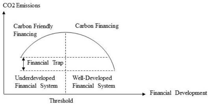
The nonlinear effect of financial development on CO2 emissions.
The variables of coc and democ were I(0) according to the first-generation unit root test of Im, Pesaran, and Shin (2003), as provided in Appendix 6. According to the second-generation unit root test of Pesaran (2007), the variables of fd, fdi, and kofgi were I(0); the variables of CO2, pols, rol, gdppc, gini, trade, infra, educ, heal, and women were I(1); the variables of pdens and urban were I(2); and the variable of wpop was I(3).
Since the working population (wpop) turned out to be I(3), the system GMM analysis covered the period 1999–2019 for 120 countries. Less than 5% of the variables were missing values. Stata's ipolate command performed the interpolation. Appendix 7 presents the correlation matrix of all variables.
3.2. Preliminary Analysis
It may be a good strategy to take into account the relationship between financial development and CO2 emissions as a static relationship by excluding the lag of CO2 emissions and the reverse causality from CO2 emissions to financial development. We only preserved the condition of a nonlinear relationship. Although this approach may be problematic due to these two exclusions, it may give us the gist of the relationship under a static setup. Hence, we estimated the main model (eq. 6) by using static panel data techniques involving fixed effect and random effect, as shown in Table 1.
| Dependent variable: d_co2 | ||
|---|---|---|
| Variable | Fixed effect | Random effect |
| fd | 0.6345** | 0.2259** |
| (0.2619) | (0.1061) | |
| fd2 | -1.1387*** | -0.4312*** |
| (0.2800) | (0.1221) | |
| constant | -0.0199 | -0.0070 |
| (0.0541) | (0.0127) | |
| Prob>F / Prob>chi2 | 0.0001 | 0.0000 |
| Observations | 2520 | 2520 |
| Countries | 120 | 120 |
| R-squared (btw) | 0.2048 | 0.2065 |
According to Table 1, financial development (fd) has a significantly positive effect, and its square (fd2) has a significantly negative effect on CO2 emissions, confirming the inverse U-curve relationship even in a static panel.
4. METHODOLOGY
Since CO2 emissions may become a self-reinforcing variable in the sense that past levels of CO2 emissions may significantly determine the current level of CO2 emissions, and the endogeneity issue may depend on the reverse causality from CO2 emissions to the main independent variable and control variables, we employed the system GMM analysis. The system GMM approach effectively addresses the challenges posed by fixed effects, heteroskedasticity, and autocorrelation. The system GMM is a suitable approach for panel data analysis when the number of groups, for instance, 120 countries in this case, exceeds the number of periods, such as 21 years.
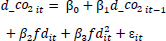
Roodman (2009) proposed the following model as the foundation for system GMM estimation:
 |
(1) |
 |
(2) |
 |
(3) |
The disturbance term εit consists of two components: µi (fixed effects) and vit (idiosyncratic shocks). These components are orthogonal to each other.
 |
(4) |
 |
(5) |
Where, wit is the instrumenting variable, which is uncorrelated with the fixed effects, E(∆witµi) is time-invariant.
The system GMM method enhances the efficiency of the estimator by introducing an additional equation (eq. 4) to the original equation (eq. 1). While the difference GMM method instruments differences using levels, the System GMM method instruments levels using differences. (Roodman, 2009). The system GMM method also assumes that there is no link between fixed effects and the first differences of instrumental variables (eq. 5). This means that the system GMM model can include more instruments than the difference GMM model.
It is essential that the idiosyncratic shocks (vit) exhibit no serial correlation. If vit is not serially correlated with order 2, then the researcher should use second and deeper lags, and if vit is serially correlated with order 2, even longer lags could be required (Roodman, 2009).
The system GMM framework uses Hansen statistics to assess the overidentification issue. It should be greater than 0.1 and less than 1.0. Therefore, the researcher should exercise caution when selecting the number of instruments.
Finally, the probability of the F statistic should be less than 0.1, which indicates the significance of the estimated model.
We estimated the effect of financial development (fd) and its square (fd2) on CO2 emissions in the main model, and made a robustness check in another four models controlling for governance variables, economic variables, social variables, and demographic variables (eq. 6-10).
Following are the reduced equation forms for each regression:
Equation for the main variable:
 |
(6) |
Equation controlling for the governance variables:
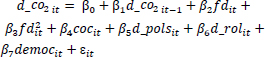 |
(7) |
Equation controlling for the economic variables:
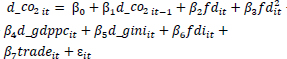 |
(8) |
Equation controlling for the social variables:
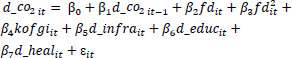 |
(9) |
Equation controlling for the demographic variables:
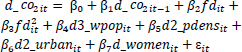 |
(10) |
Stata’s xtabond2 package of system GMM analysis proposed by Roodman (2009) was used for the main analysis. The codes used in Stata are provided in Appendix 8 for replication.
5. RESULTS AND DISCUSSION
The exogenous and endogenous variables should be determined before conducting system GMM analysis since endogeneity means that there exists a reverse causality stemming from the dependent variable to the independent variables (Gök & Sodhi, 2021). The results in Appendix 4 indicate that we treated all variables endogenously.
Table 2 shows that the estimated models made sense because their Prob>F was less than 0.1, sometimes even 0.000; the Hansen p-values were over 0.1; and the AR(3) p-values were over 0.1 and not equal to 1.0, which means that the right number of lags were used (fourth and deeper lags have been instrumented for the regressions).
According to Table 2, the lag of CO2 emissions (l.d_co2) had a significantly negative impact on the current level of CO2 emissions (d_co2). Hence, CO2 emissions were not a self-reinforcing variable; instead, the past level of CO2 emissions was an important determinant of the current level of CO2 emissions due to strategic substitution between past and current levels of CO2 emissions. The fact that the lag of CO2 emissions had a significantly negative effect shows that countries quickly reached their steady-state level of CO2 emissions. It also indicates that improvement or disimprovement in CO2 emissions is challenging in the short run since yearly data have been provided. Any improvement in the previous year leads to a decrease in the following year, and vice versa. Governments allocating resources to reduce CO2 emissions in the last year have a smaller amount of resources to allocate in the current year, so CO2 emissions rise. The result also indicates the persistence of systematic barriers that prevent countries from reducing CO2 emissions since the decreasing amount of CO2 emissions in the previous year does not lead to decreasing CO2 emissions in the next year. We have also made an attempt to explain these systematic barriers.
| Dependent variable: d_co2 | |||||
|---|---|---|---|---|---|
| Variable | Main | Governance | Economic | Social | Demographic |
| l.d_co2 | -0.1297*** | -0.1993*** | -0.2002*** | -0.2825*** | -0.2575*** |
| (0.0161) | (0.0706) | (0.0301) | (0.0137) | (0.0464) | |
| fd | 1.5725*** | 3.3656** | 3.4237*** | 5.0087*** | 2.7217*** |
| (0.3580) | (1.3892) | (0.7636) | (0.4097) | (0.8927) | |
| fd2 | -2.1912*** | -4.1768*** | -3.8960*** | -4.8772*** | -3.5426*** |
| (0.3556) | (1.4662) | (0.8225) | (0.3716) | (0.9529) | |
| coc | 0.0234 | ||||
| (0.1672) | |||||
| d_pols | -0.7675*** | ||||
| (0.2184) | |||||
| d_rol | -1.8984*** | ||||
| (0.5330) | |||||
| democ | 0.2871* | ||||
| (0.1585) | |||||
| d_gdppc | 2.45e-04*** | ||||
| (2.41e-05) | |||||
| d_gini | 0.0879** | ||||
| (0.0428) | |||||
| fdi | -0.0015*** | ||||
| (0.0003) | |||||
| d_trade | -0.0037*** | ||||
| (0.0010) | |||||
| kofgi | -0.0254*** | ||||
| (0.0020) | |||||
| d_infra | 0.0516*** | ||||
| (0.0052) | |||||
| d_educ | 0.0631 | ||||
| (0.0664) | |||||
| d_heal | 0.6757*** | ||||
| (0.1206) | |||||
| d3_wpop | 0.7789*** | ||||
| (0.2951) | |||||
| d2_pdens | -0.0318 | ||||
| (0.0493) | |||||
| d2_urban | -2.4240*** | ||||
| (0.6392) | |||||
| d_women | -0.0323** | ||||
| (0.0140) | |||||
| constant | -0.1652** | -0.4129* | -0.4638*** | 0.6330*** | -0.2799** |
| (0.0629) | (0.2438) | (0.1224) | (0.0984) | (0.1378) | |
| Prob>F | 0.000 | 0.000 | 0.000 | 0.000 | 0.000 |
| Observations | 2400 | 2400 | 2400 | 2400 | 2400 |
| Countries | 120 | 120 | 120 | 120 | 120 |
| Instruments | 46 | 33 | 43 | 79 | 42 |
| Hansen | 0.130 | 0.801 | 0.159 | 0.127 | 0.304 |
| AR(3) | 0.125 | 0.109 | 0.143 | 0.140 | 0.136 |
| Specification: f(x)=x^2 | ||
|---|---|---|
| Extreme point: 0.3588 | ||
| Lower bound | Upper bound | |
| Interval | 0.02 | 1 |
| Slope | 1.48 | -3.81 |
| t-value | 4.3162 | -8.6892 |
| P>|t| | 1.65E-05 | 2.35E-12 |
| Overall test of the presence of an inverse U-shape. | ||
| t-value | 4.32 | |
| P>|t| | 1.65E-05 | |
Financial development (fd) has been found to have a significantly positive effect on CO2 emissions (d_co2) and the square of financial development (fd2) has been found to have a significantly negative effect on CO2 emissions (d_co2), both supporting our main hypothesis of the modified Kuznets Curve relationship (Akca, 2021; Balaguer & Cantavella, 2016; Dinda, 2004; Stern, 2018). The results have been found to be robust with respect to the estimation results of other specifications. Also, Table 3 indicates the presence of an inverse U-curve relationship between financial development and CO2 emissions.
The results obtained with respect to the governance variables are as follows: political stability (d_pols) has been found to have a significantly negative effect on CO2 emissions (CO2). A politically stable government is more likely to enact consistent policies and laws that support CO2 reduction by providing long-term incentives for renewable energy development while discouraging the use of fossil fuels. Political stability may reduce the uncertainties and risks associated with clean energy investment for the development of sustainable technologies. Political stability can promote international collaboration and coordination to address climate change, resulting in more effective global efforts to cut CO2 emissions. Rule of law (d_rol) has been found to have a significantly negative effect on CO2 emissions (CO2). The rule of law makes it possible to enforce environmental laws effectively by issuing fines and penalties for not following the rules. This can be a strong deterrent for actions that hurt the environment and a motivator for businesses to adopt environmentally friendly methods. The rule of law encourages transparency and involvement in environmental decision-making processes, which may serve to guarantee that environmental laws and regulations are effective, fair, and equitable by fostering trust among government, corporations, and individuals. Democracy (democ) has been found to have a significantly positive effect on CO2 emissions (d_co2). The advantages of democracy are not distributed equitably between investors and ordinary individuals. Investors, in partnership with powerful elites, have the right not just to safeguard their property rights, but also to pollute against the common benefit of society. The power dynamics between investors and the government outweigh the public voice of individuals and non-governmental organizations (NGOs). Although individuals and NGOs want less pollution, their voices cannot be heard by the government and the Senate against Hobbesian investors who collaborate with powerful elites (Gök, 2020). This supports the empirical findings of Gök (2020).
The results obtained with respect to the economic variables are highlighted as follows: income per capita (gdppc) has been found to have a significantly positive effect on CO2 emissions (d_co2). As countries experience industrialization and economic growth in terms of higher income per capita, they tend to consume more energy mainly derived from fossil fuels, which leads to an increase in CO2 emissions. Governments may pursue less stringent environmental regulations and policies for the sake of higher income per capita, resulting in higher economic growth rates. Income inequality (d_gini) has been observed to have a significantly positive effect on CO2 emissions (d_co2). Jorgenson et al. (2017) found higher income concentrations at the top of the income distribution to lead to more competition in consumption and longer work hours. This phenomenon, known as the Veblen effect, leads to an increase in energy consumption and CO2 emissions, as wealthy individuals purchase expensive public goods and services to flaunt their wealth, while low-income households increase their spending to match the lifestyles of their wealthier counterparts. Lower-income households increase their average working hours to keep up with the induced status spending, resulting in increased energy consumption and emissions (Jebli, M. B., 2016; Pao & Tsai, 2011). This result supported the empirical findings of Jorgenson et al. (2016, 2017) and Baek and Gweisah (2013); however, it did not support the empirical findings obtained by Demir, Cergibozan, and Gök (2019). Foreign direct investment inflows (fdi) have been found to have a significantly negative effect on CO2 emissions (d_co2). Multinational companies (MNCs) often introduce green technologies to their host countries, thereby reducing CO2 emissions. FDI may lead to the upgrading of infrastructure in host countries, resulting in more efficient transportation systems or energy-efficient buildings. MNCs may propose superior management techniques to the host countries, resulting in more efficient and sustainable utilization of resources. International trade, or trade openness (d_trade), has been observed to have a significantly negative effect on CO2 emissions (d_co2). International trade allows countries to specialize in the production of goods and services in which they are most efficient, which may lead to higher productivity, lower costs, and less waste, resulting in lower CO2 emissions. International trade allows countries to take advantage of their comparative advantages by producing and exporting goods and services that require fewer emissions to produce while importing products and services that require more emissions to produce, which may lead to a decrease in global CO2 emissions.
The results acquired with reference to the social variables are as follows: globalization (kofgi) has been found to have a significantly negative effect on CO2 emissions (d_co2). Globalization may stimulate the use of more efficient production technology, leading to lower energy consumption and CO2 emissions (KOF SEI, 2022). As countries become more interconnected via trade and investment, there is increased opportunity for innovation and the sharing of innovative technology that can reduce CO2 emissions. Globalization may also ease the cross-border movement of renewable energy technology and resources, helping countries shift away from fossil fuels toward cleaner energy sources. Infrastructure (d_infra) has been observed to positively affect CO2 emissions (d_co2). Infrastructure projects often need large amounts of building materials, like steel and concrete, that have high carbon footprints. Manufacturing these materials requires the use of fossil fuels, increasing CO2 emissions. Large amounts of energy, often derived from fossil fuels, are required for the construction and operation of highways, airports, and buildings, resulting in higher CO2 emissions. Infrastructure projects frequently require deforestation or land clearing, which may result in higher CO2 emissions. Health (d_heal) has been found to have a significantly positive effect on CO2 emissions (d_co2). Living a healthier and longer life requires more medical attention, leading to an increase in healthcare activities, such as hospital visits, medical tests, and surgeries, which require a significant amount of energy, including electricity, heating, and cooling, leading to higher CO2 emissions. The production and transportation of medications require energy, which is mainly derived from fossil fuels, leading to higher CO2 emissions. As healthcare improves, the use of medical waste, such as disposable gloves, masks, and syringes, increases, which leads to higher CO2 emissions since these items are often made from plastic, and it requires energy to manufacture and dispose them properly.
The results obtained with respect to the demographic variables are as follows. The working population (d3_wpop) has been found to have a significantly positive effect on CO2 emissions (d_co2). As the working population grows, more individuals may need to commute to and from work, which may increase the number of vehicles on the road, leading to higher CO2 emissions. More office buildings are also required to accommodate the growing number of workers. The increase in heating, cooling, lighting, and running office equipment requires a significant amount of energy, leading to higher CO2 emissions. Urbanization (d2_urban) has been found to have a significantly negative effect on CO2 emissions (d_co2). People tend to live densely in smaller homes or apartments in urban areas in which less energy is required for heating and cooling, which may lead to lower CO2 emissions. Compared to suburban or rural areas, urban structures may have stricter energy efficiency standards, leading to buildings using less energy for lighting, heating, and cooling, which might result in lower CO2 emissions. Better transportation alternatives, including trains, buses, and subways, are frequently found in urban areas, which may decrease the demand for private cars, resulting in lower transportation-related CO2 emissions. The representation of women in parliament (d_women) has also been found to significantly reduce CO2 emissions (d_co2). Women in parliament are more likely to support and speak out in favor of sustainable policies and projects that can lower CO2 emissions, such as renewable energy, public transportation, and energy efficiency. Women leaders are more inclined to engage in international cooperation and collaboration to address climate change due to their stronger and more coordinated efforts to reduce global CO2 emissions.
CONCLUSION
We established a nonlinear theory to investigate the effect of financial development on CO2 emissions by reconciling four hypotheses, including carbon-friendly financing, carbon financing, pollution haven, and pollution halo. The main assumption of the theory is that the effect of financial development on CO2 emissions depends on whether there exists an underdeveloped financial system or a well-developed financial system in the country.
In countries with underdeveloped financial systems, the financial system provides credits, and the government provides incentives to carbon-emitting industries, which is referred to as carbon-friendly financing. As a result of these less stringent environmental regulations, multinational firms or foreign investors relocate their production to these countries, a phenomenon referred to as pollution haven. In countries with strong financial systems, the government and financial systems offer credits and incentives to low-carbon or non-carbon industries. This is called “carbon financing”, and strict environmental rules cause multinational companies, or foreign investors, to move their production out of these countries. This is called “pollution halo”.
Then we further developed our hypothesis, which consisted of two sub-hypotheses: below the specific threshold of financial development, financial development has a significantly positive effect on CO2 emissions as carbon-friendly financing in underdeveloped financial systems. Above the specific threshold of financial development, financial development has a significantly negative effect on CO2 emissions as carbon financing in well-developed financial systems.
Our theory also introduced the concept of a financial trap, where countries with underdeveloped financial systems consistently exhibit higher CO2 emission levels than those with well-developed financial systems.
We used system GMM analysis to test our hypothesis and found a U-shaped inverse relationship between financial development and CO2 emissions for 120 countries from 1999 to 2019. The result turned out to be robust when we compared the result of the main model with the other four models.
POLICY IMPLICATIONS
To overcome the financial trap, countries with weak financial systems need to build or strengthen regulatory frameworks to keep the system stable, honest, and effective. This can be done by setting rules and oversight mechanisms that encourage financial institutions to be open, accountable, and good at managing risks. Regulatory frameworks should also be accessible and understandable for those concerned, and compliance with these rules should be mandatory. Effective and continuous audit mechanisms should be put in place to monitor compliance and eliminate potential risks. Mechanisms to hold the financial system's stakeholders accountable for their actions and transactions should also be developed. These mechanisms should include penalizing misconduct, deterring risks, and effective whistleblowing methods. Governments should encourage financial institutions to implement robust risk management frameworks to conduct comprehensive risk assessments, diversify their portfolios, and increase their resilience to adverse scenarios.
With regard to countries with strong financial systems, policymakers should ensure the creation and implementation of green finance or carbon finance initiatives to support investments that are good for the environment. These initiatives can include giving banks reasons to invest in low-carbon technologies and projects, setting up green bonds or funds, and encouraging environmental risk assessments to be used in financial decision-making. To help these countries find other solutions, institutions could include environmental risk assessments in the decisions they make regarding money. These are needed to figure out how climate change, limited natural resources, and other environmental factors might affect their assets and debts. All of these steps would not only speed up the switch to a green economy in countries with strong financial systems, but it would also make it possible to build a society free of environmental problems (Zhang et al., 2022).
All countries should implement carbon pricing mechanisms, such as carbon taxes or emissions trading systems, which may provide economic incentives for businesses and individuals to reduce their carbon emissions. These mechanisms can be designed to encourage financial institutions to invest in low-carbon projects and provide support for the transition to a low-carbon economy. High carbon taxes on emission-intensive sectors could reduce carbon-intensive practices and become financial incentives for businesses and individuals, helping them switch to low-carbon technologies. Using the money from carbon taxes to fund projects, like energy efficiency or renewable energy subsidies, and backing them up with other policies could also make a big difference in reaching long-term climate goals.
AUTHORS’ CONTRIBUTIONS
The authors confirm their contribution to the paper as follows: data analysis and interpretation, drafting of the manuscript, and revision of the manuscript: A.G.; conceptualization and writing of the manuscript: T.Y., E.S. All authors have reviewed the results and approved the final version of the manuscript.
LIST OF ABBREVIATIONS
| GHG | = Green House Gas |
| FD | = financial Development |
| MNCs | = Multinational Companies |
AVAILABILITY OF DATA AND MATERIALS
The data and supportive information are available within the article.
ACKNOWLEDGEMENTS
Declared none.
APPENDIX
| Albania | Costa Rica | Israel | Norway |
| Algeria | Cote d'Ivoire | Italy | Oman |
| Angola | Croatia | Japan | Pakistan |
| Argentina | Cyprus | Jordan | Panama |
| Armenia | Czechia | Kazakhstan | Peru |
| Australia | Denmark | Kenya | Philippines |
| Austria | Dominican Rep. | Korea, Rep. | Poland |
| Azerbaijan | Ecuador | Kyrgyz Rep. | Portugal |
| Bangladesh | Egypt, Arab Rep. | Lao PDR | Romania |
| Barbados | El Salvador | Latvia | Russian Federation |
| Belarus | Estonia | Lithuania | Rwanda |
| Belgium | Eswatini | Luxembourg | Senegal |
| Belize | Finland | Madagascar | Slovak Republic |
| Benin | France | Malaysia | Slovenia |
| Bhutan | Gabon | Mali | South Africa |
| Botswana | Gambia | Malta | Spain |
| Brazil | Georgia | Mauritania | Sudan |
| Bulgaria | Germany | Mauritius | Sweden |
| Burkina Faso | Ghana | Mexico | Switzerland |
| Burundi | Greece | Mongolia | Tajikistan |
| Cabo Verde | Guatemala | Morocco | Tanzania |
| Cambodia | Guinea | Mozambique | Thailand |
| Cameroon | Guyana | Namibia | Togo |
| Canada | Honduras | Nepal | Tunisia |
| Central African Rep. | Hungary | Netherlands | Turkiye |
| Chad | Iceland | New Zealand | Uganda |
| Chile | India | Nicaragua | Ukraine |
| China | Indonesia | Niger | United Kingdom |
| Colombia | Iran, Islamic Rep. | Nigeria | United States |
| Comoros | Ireland | North Macedonia | Uruguay |
| Variable | Definition | Source |
|---|---|---|
| CO2 | CO2 emissions (metric tons per capita) | WDI (2023) |
| Fd | Financial development index | IMF (2023) |
| Governance variables | ||
| Coc | Control of corruption: estimate | WGI (2023) |
| pols | Political stability and absence of violence/terrorism: estimate | WGI (2023) |
| rol | Rule of law: estimate | WGI (2023) |
| democ | Voice and accountability: estimate | WGI (2023) |
| Economic variables | ||
| gdppc | GDP per capita (constant 2015 US$) | WDI (2023) |
| gini | gini_disp | Solt (2020) |
| fdi | Foreign direct investment, net inflows (% of GDP) | WDI (2023) |
| trade | Trade (% of GDP) | WDI (2023) |
| Social variables | ||
| kofgi | KOF globalisation index | KOF SEI (2022) |
| infra | Fixed broadband subscriptions (per 100 people) | WDI (2023) |
| educ | Principal component analysis of the following variables: | |
| School enrollment, primary (% gross) | WDI (2023) | |
| School enrollment, secondary (% gross) | WDI (2023) | |
| School enrollment, tertiary (% gross) | WDI (2023) | |
| heal | Principal component analysis of the following variables: | |
| Life expectancy at birth, total (years) | WDI (2023) | |
| 1000 - mortality rate, infant (per 1,000 live births) | WDI (2023) | |
| Physicians (per 1,000 people) | WDI (2023) | |
| Demographic variables | ||
| wpop | Population aged 15-64 (% of total population) | WDI (2023) |
| pdens | Population density (people per sq. km of land area) | WDI (2023) |
| urban | Urban population (% of total population) | WDI (2023) |
| women | Proportion of seats held by women in national parliaments (%) | WDI (2023) |
| Variable | Obs. | Mean | Std. dev. | Min. | Max. |
|---|---|---|---|---|---|
| CO2 | 2880 | 4.169 | 4.347 | 0 | 25.604 |
| fd | 2880 | 0.336 | 0.246 | 0 | 1 |
| coc | 2880 | 0.065 | 1.034 | -1.597 | 2.459 |
| pols | 2880 | -0.031 | 0.942 | -2.810 | 1.758 |
| rol | 2880 | 0.062 | 0.996 | -1.841 | 2.124 |
| democ | 2880 | 0.110 | 0.951 | -1.858 | 1.800 |
| gdppc | 2880 | 13116. 270 | 18351.270 | 234.709 | 112417.900 |
| gini | 2880 | 38.756 | 8.832 | 21.900 | 65.300 |
| fdi | 2880 | 5.305 | 18.035 | -57.532 | 449.080 |
| trade | 2880 | 80.610 | 45.163 | 1.218 | 377.843 |
| kofgi | 2880 | 61.237 | 16.077 | 22 | 91 |
| infra | 2880 | 7.494 | 11.614 | 0 | 46.906 |
| educ | 2880 | 0 | 0.972 | -3.848 | 3.727 |
| heal | 2880 | 0 | 1.607 | -4.715 | 2.962 |
| urban | 2880 | 57.350 | 21.829 | 7.412 | 98.041 |
| wpop | 2880 | 62.261 | 6.474 | 47.386 | 75.369 |
| pdens | 2880 | 127.348 | 188.751 | 1.523 | 1575.194 |
| women | 2880 | 18.077 | 11.290 | 0 | 63.750 |
| Dependent variable: CO2 | ||
|---|---|---|
| Independent variables | Z-bar | Z-bar tilde |
| Fd | 15.882* | 12.406* |
| Coc | 8.286* | 6.133* |
| pols | 10.861* | 8.259* |
| Rol | 7.741* | 5.682* |
| democ | 3.811* | 2.436* |
| gdppc | 11.043* | 8.409* |
| gini | 39.325* | 31.768* |
| fdi | 6.623* | 4.759* |
| trade | 15.233* | 11.870* |
| kofgi | 2.764* | 1.572 |
| infra | 40.638* | 32.852* |
| educ | 22.845* | 18.157* |
| heal | 26.236* | 20.957* |
| urban | 63.783* | 51.967* |
| wpop | 214.591* | 176.519* |
| pdens | 71.039* | 57.960* |
| women | 9.251* | 6.930* |
| Variable | CD-test | p-value |
|---|---|---|
| CO2 | 27.749 | 0.000 |
| fd | 156.849 | 0.000 |
| coc | -1.406 | 0.160 |
| pols | 16.619 | 0.000 |
| rol | 14.001 | 0.000 |
| democ | 1.897 | 0.058 |
| gdppc | 296.390 | 0.000 |
| gini | 13.441 | 0.000 |
| fdi | 37.461 | 0.000 |
| trade | 69.067 | 0.000 |
| kofgi | 371.599 | 0.000 |
| infra | 348.168 | 0.000 |
| educ | 196.512 | 0.000 |
| heal | 373.329 | 0.000 |
| wpop | 106.835 | 0.000 |
| pdens | 218.803 | 0.000 |
| urban | 230.714 | 0.000 |
| women | 235.597 | 0.000 |
| Im, Pesaran and Shin (2003) | ||||||||
|---|---|---|---|---|---|---|---|---|
| Level | First difference | Second difference | Third difference | |||||
| Constant | Constant | Constant | Constant | |||||
| Variable | Constant | &Trend | Constant | &Trend | Constant | &Trend | Constant | &Trend |
| coc | -3.724* | -3.867* | ||||||
| democ | -7.173* | -5.271* | ||||||
| Pesaran (2007) | ||||||||
| Level | First difference | Second difference | Third difference | |||||
| Constant | Constant | Constant | Constant | |||||
| Variable | Constant | &Trend | Constant | &Trend | Constant | &Trend | Constant | &Trend |
| CO2 | -1.069 | -2.681* | -4.514* | -4.640* | ||||
| fd | -2.505* | -3.016* | ||||||
| pols | -2.178* | -2.415 | -4.529* | -4.584* | ||||
| rol | -1.934 | -2.264 | -4.224* | -4.345* | ||||
| gdppc | -1.383 | -1.633 | -3.008* | -3.431* | ||||
| gini | -0.932 | -1.489 | -2.649* | -2.961* | ||||
| fdi | -3.265* | -3.639* | ||||||
| trade | -1.489 | -2.211 | -3.992* | -4.090* | ||||
| kofgi | -3.583* | -2.840* | ||||||
| infra | -2.021 | -1.917 | -3.205* | -3.665* | ||||
| educ | -1.642 | -1.984 | -3.676* | -3.667* | ||||
| heal | -1.723 | -1.990 | -3.687* | -4.104* | ||||
| wpop | -1.213 | -1.173 | -1.380 | -1.618 | -2.366* | -2.497 | -3.641* | -3.611* |
| pdens | -0.940 | -1.209 | -1.600 | -1.993 | -3.240* | -3.346* | ||
| urban | -0.639 | -1.009 | -1.295 | -2.538 | -3.862* | -4.078* | ||
| women | -2.014 | -2.343 | -4.304* | -4.348* | ||||
| d_co2 | fd | fd2 | coc | d_pols | d_rol | democ | d_gdppc | d_gini | fdi | |
|---|---|---|---|---|---|---|---|---|---|---|
| d_co2 | 1.0000 | |||||||||
| fd | -0.0811 | 1.0000 | ||||||||
| fd2 | -0.0918 | 0.9674 | 1.0000 | |||||||
| coc | -0.0978 | 0.7758 | 0.7451 | 1.0000 | ||||||
| d_pols | 0.0018 | -0.0190 | -0.0181 | -0.0097 | 1.0000 | |||||
| d_rol | -0.0452 | -0.0183 | -0.0168 | 0.0002 | 0.1982 | 1.0000 | ||||
| democ | -0.1045 | 0.6953 | 0.6464 | 0.8323 | -0.0128 | -0.0227 | 1.0000 | |||
| d_gdppc | 0.1023 | 0.2950 | 0.2822 | 0.3180 | 0.0575 | 0.0368 | 0.2882 | 1.0000 | ||
| d_gini | -0.0233 | 0.0517 | 0.0664 | 0.0842 | -0.0130 | -0.0098 | 0.0522 | 0.0057 | 1.0000 | |
| fdi | -0.0099 | 0.0777 | 0.0567 | 0.1006 | -0.0074 | 0.0012 | 0.1155 | 0.0670 | 0.0034 | 1.0000 |
| d_trade | 0.0470 | 0.0336 | 0.0339 | 0.0644 | -0.0112 | 0.0165 | 0.0780 | 0.1679 | 0.0153 | 0.1239 |
| kofgi | -0.1046 | 0.8196 | 0.7393 | 0.7290 | -0.0096 | 0.0053 | 0.7538 | 0.2946 | 0.0225 | 0.1150 |
| d_infra | -0.0082 | 0.4705 | 0.4382 | 0.4404 | -0.0108 | 0.0303 | 0.4209 | 0.2499 | 0.0275 | 0.1406 |
| d_educ | 0.0279 | -0.0973 | -0.0757 | -0.0642 | 0.0098 | 0.0108 | -0.0775 | -0.0134 | 0.0442 | -0.0059 |
| d_heal | 0.0293 | -0.2118 | -0.1798 | -0.1758 | 0.0318 | 0.0237 | -0.2032 | -0.0620 | 0.0169 | -0.0176 |
| d2_urban | 0.0013 | -0.0374 | -0.0334 | -0.0254 | -0.0271 | -0.0149 | -0.0129 | 0.0091 | 0.0254 | -0.0252 |
| d3_wpop | -0.0408 | 0.0241 | 0.0199 | 0.0142 | -0.0012 | 0.0063 | 0.0206 | 0.0089 | -0.0081 | -0.0198 |
| d2_pdens | -0.0092 | 0.0052 | 0.0019 | 0.0097 | 0.0233 | 0.0099 | 0.0135 | 0.0418 | 0.0051 | -0.0049 |
| d_women | -0.0011 | -0.0165 | -0.0116 | -0.0194 | 0.0445 | 0.0495 | -0.0155 | -0.0096 | -0.0162 | -0.0123 |
| d_trade | kofgi | d_infra | d_educ | d_heal | d2_urban | d3_wpop | d2_pdens | d_women | |
|---|---|---|---|---|---|---|---|---|---|
| d_trade | 1.0000 | ||||||||
| kofgi | 0.0534 | 1.0000 | |||||||
| d_infra | 0.0492 | 0.5064 | 1.0000 | ||||||
| d_educ | -0.0004 | -0.1433 | -0.0784 | 1.0000 | |||||
| d_heal | -0.0041 | -0.2790 | -0.1098 | 0.0533 | 1.0000 | ||||
| d2_urban | 0.0260 | -0.0329 | -0.0304 | 0.0057 | -0.0168 | 1.0000 | |||
| d3_wpop | -0.0371 | 0.0392 | 0.0097 | -0.0084 | -0.0075 | -0.0242 | 1.0000 | ||
| d2_pdens | -0.0016 | 0.0128 | -0.0138 | 0.0292 | 0.0187 | -0.0050 | 0.0109 | 1.0000 | |
| d_women | 0.0267 | -0.0128 | -0.0207 | 0.0102 | 0.0271 | -0.0380 | -0.0044 | 0.0047 | 1.0000 |
| xtset id year |
| sum |
| For creating education variable with PCA: |
| pca pse sse tse |
| predict pc1 pc2 pc3 |
| gen educ=pc1*0.6297/0.9433+pc2*0.3136/0.9433 |
| For creating health variable with PCA: |
| pca life imort phy |
| predict pc1 pc2 pc3 |
| gen heal=pc1 |
| To test cross-section independence: |
| xtcdf co2 fd coc pols rol democ gdppc gini fdi trade kofgi infra educ heal urban wpop pdens women |
| For second-generation unit root test: |
| xtcips co2, maxlags(1) bglags(1) |
| xtcips co2, maxlags(1) bglags(1) trend |
| xtcips d.co2, maxlags(1) bglags(1) |
| xtcips d.co2, maxlags(1) bglags(1) trend |
| … |
| For Granger non-causality test: |
| xtgcause fd co2 |
| xtgcause coc co2 |
| … |
| For system GMM: |
| xtabond2 d_co2 l.d_co2 fd fd2, gmm(d_co2 fd fd2, collapse lag(4 17)) artests (8) small twostep |
| utest fd fd2 |
| xtabond2 d_co2 l.d_co2 fd fd2 coc d_pols d_rol democ, gmm(d_co2 fd fd2 d_pols d_rol democ, collapse lag(4 7)) gmm(coc, collapse lag(4 4)) artests (8) small twostep |
| utest fd fd2 |
| … |

